Performing simple linear regressions in R

Linear regression

We will use the mtcars data, specifically the miles per gallon (mpg) versus the weight (wt) - we obviously expect to see a strong association between these two variables.

fit <- lm(mpg~wt, data=mtcars)
summary(fit)

## 
## Call:
## lm(formula = mpg ~ wt, data = mtcars)
## 
## Residuals:
##     Min      1Q  Median      3Q     Max 
## -4.5432 -2.3647 -0.1252  1.4096  6.8727 
## 
## Coefficients:
##             Estimate Std. Error t value Pr(>|t|)    
## (Intercept)  37.2851     1.8776  19.858  < 2e-16 ***
## wt           -5.3445     0.5591  -9.559 1.29e-10 ***
## ---
## Signif. codes:  0 '***' 0.001 '**' 0.01 '*' 0.05 '.' 0.1 ' ' 1
## 
## Residual standard error: 3.046 on 30 degrees of freedom
## Multiple R-squared:  0.7528, Adjusted R-squared:  0.7446 
## F-statistic: 91.38 on 1 and 30 DF,  p-value: 1.294e-10

Plotting

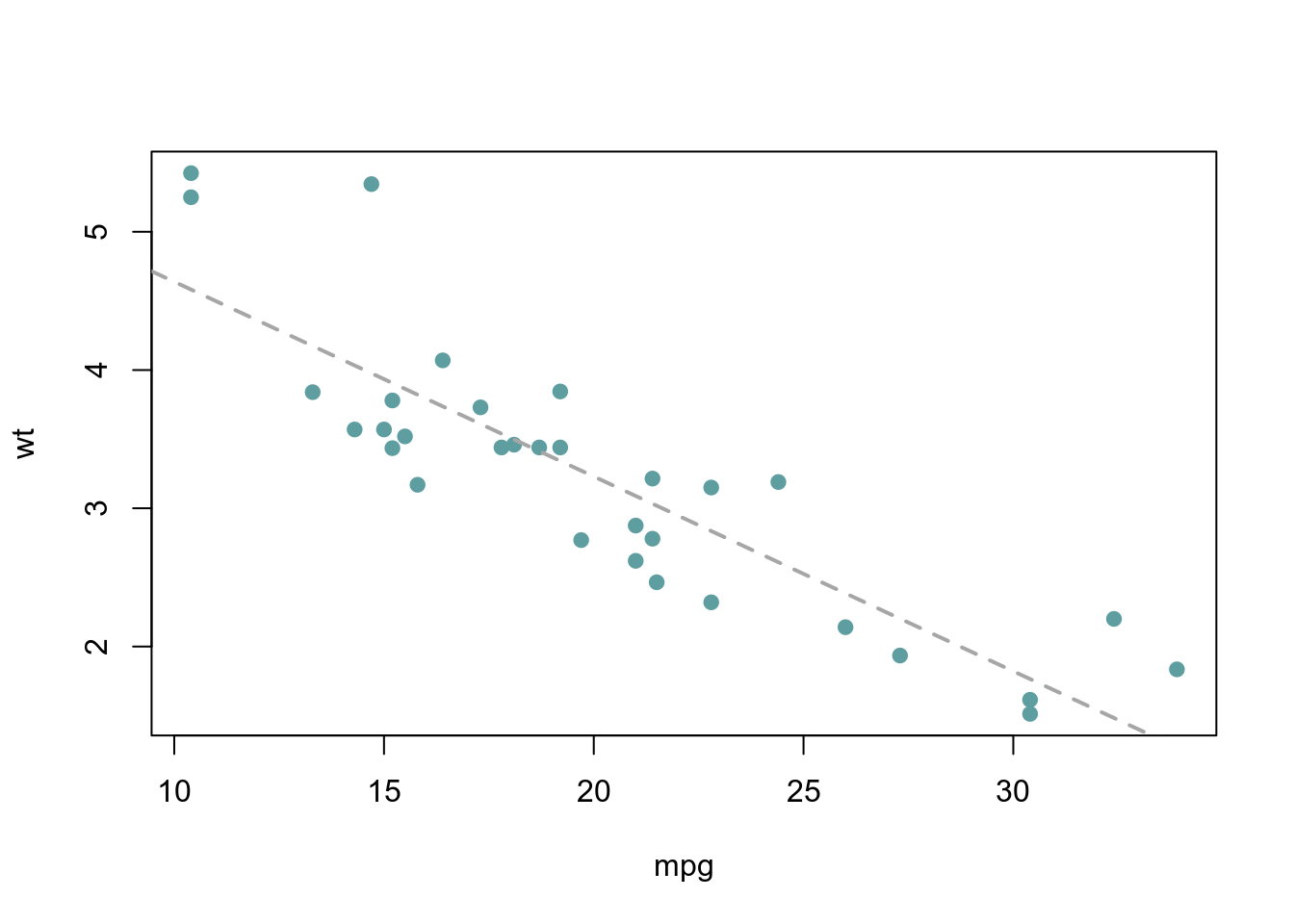
We can create a simple scatter plot of mpg vs wt an then fit the regression line to this:

plot(mtcars$mpg, mtcars$wt, pch = 19, col = 'cadetblue', xlab = 'mpg', ylab = 'wt')
abline(lm(wt~mpg, data=mtcars), lty = 2, lwd = 2, col = 'grey65')